Line fitting to a set of 2D points

Goal

In this tutorial you will learn how to fit the some set of 2D points by using the algorithms of Robest.

Task details

You have a set of 2d points, some of which (inliers) follow some rectilinear law. However, the data are quite corrupted and among all points there are so-called outliers. Thus, the main task is reduced to the definition of this linear law and the search for inliers in the set of points.

A set of 2D points is presented in the form of a table Excel.

Code

The tutorial code’s is shown lines below.

#include <sstream>
#include <string>
#include <fstream>

#include "LineFitting/LineFitting.hpp"

int main()
{
    // ***** Part 1: Reading the data.

    std::vector<double> x;
    std::vector<double> y;

    std::ifstream file( "/DatasetOfPoints.csv" );
    std::string line = "";
    std::string value = "";

    while (getline(file, line))
    {
        value = "";
        for (int i = 0; i < line.size(); i++)
        {
            if (line[i] == ',' && i != 0)
                x.push_back(atof(value.c_str()));

            if (i == line.size() - 1 && i != 0)
                y.push_back(atof(value.c_str()));

            line[i] != ',' ? value += line[i]:value = "";
        }
    }
    file.close();

    // ***** Part 2: Define estimation problem.

    LineFittingProblem * lineFitting = new LineFittingProblem();
    lineFitting->setData(x,y);

    // ***** Part 3: Solve.

    robest::MSAC * MSACsolver = new robest::MSAC();
    MSACsolver->solve(lineFitting,0.02);

    // ***** Part 4: Get parametres of the model.

    double res_k,res_b;
    lineFitting->getResult(res_k,res_b);

    std::cout << std::endl;
    std::cout << "Best model is: y = " << res_k << "*x + " << res_b;
    std::cout << std::endl;

    return 0;
}

Explanation

• Including libraries

  // tools for working with files
  #include <sstream>
  #include <string>
  #include <fstream>
  
  // line fitting algorithm
  #include "LineFitting/LineFitting.hpp"
  

• Reading data set

  int main()
  {
      // ***** Part 1: Reading the data.
  
      std::vector<double> x;  // vector of x coordiantes
      std::vector<double> y;  // vector of y coordiantes
  
      // reading the file
      std::ifstream file( "/DatasetOfPoints.csv" );
      std::string line = "";
      std::string value = "";
  
      // filling vectors
      while (getline(file, line))
      {
          value = "";
          for (int i = 0; i < line.size(); i++)
          {
              if (line[i] == ',' && i != 0)
                  x.push_back(atof(value.c_str()));
  
              if (i == line.size() - 1 && i != 0)
                  y.push_back(atof(value.c_str()));
  
              line[i] != ',' ? value += line[i]:value = "";
          }
      }
      file.close();
  

• Estimation problem initialization

  // ***** Part 2: Define estimation problem.
  
  LineFittingProblem * lineFitting = new LineFittingProblem();
  lineFitting->setData(x,y);
  

• Choosing the parameters of estimation algorithm

  As the main algorithm, we will use MSAC. At the input, this method accepts a pointer to the estimation function, a threshold value for determining the inliers, and also the number of iterations for which the model should be fitted.

  As a pointer, we have already defined the fit of the lineFitting. The threshold value will be 0.02. And to select the number of iterations, there are two ways:

  First way: we can manually set the value of the number of iterations.

  The second way: we can use the default value. It is calculated according to the following formula:

  \[nbIter = \frac { log(1 - p) }{ log(1 - w^n) }\]

  Where p is the probability of successful completion of the algorithm, w is the inliers ratio, n is the size of the data set.

  It is worth noting that if the value of the number of iterations obtained as a result of automatic calculation will exceed 50000, the function calculateIterationsNb will return the value of 50000.

• Solving and analyse the results

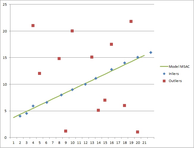
      // ***** Part 3: Solve.
  
      robest::MSAC * MSACsolver = new robest::MSAC();
      MSACsolver->solve(lineFitting,0.02);     // threshold = 0.02
  
      // ***** Part 4: Get parametres of the model.
  
      double res_k,res_b;
      lineFitting->getResult(res_k,res_b);
  
      std::cout << std::endl;
      std::cout << "Best model is: y = " << res_k << "*x + " << res_b;
      std::cout << std::endl;
  
      return 0;
  }
  

  As parameters, the algorithm returns two values. So, a linear law describing a given set of 2D points takes the following form:

  \[y(x) = 5.83333x + 3.16667\]

  In order to demonstrate the correctness of the calculated model, we will use Excel. The result is shown in the figure below.